In the previous article we discussed how we can use reinforcement learning to design simple architectures like some types of convolutional neural networks. Today I am bringing to you the explanation on how to design more complex architectures. Before diving into how to modify the controller, let’s introduce another way of thinking about recurrent nertworks. Typically, LSTM and GRU are explained through formulas or diagrams like the one I showed in the previous article. However, in the NAS paper they introduced another way of thinking about them. They used a graph representation in which states are nodes, and the edges represent the way of merging states. For instance, and edge can mean to apply a sigmoid function, another can be summing two hidden states, and so on. Below is a simple example visualized.

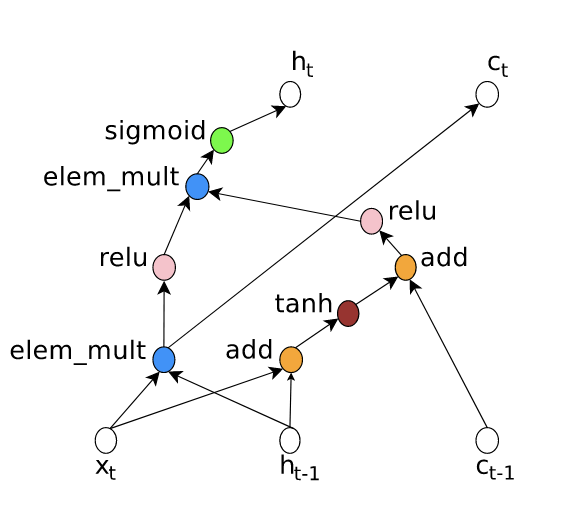
Here the input is $x_t$, the hidden state from the previous step $h_{t-1}$ and the cell state $c_{t-1}$ which is used as memory. As you can see the states are combined either using multiplication or addition, and then some activation functions are applied. Now, think for a moment how can you represent this same graph in a linear way, as a sequence of operations. You have it? Well, one possible way would be [Add, Tanh, Multiply, ReLU, Multiply, sigmoid, Add, ReLU, 1, 0]. Don’t worry, there are many ways to represent the above graph sequentally, this one is just the one provided by the author of the NAS. To understand it look at the next picture.

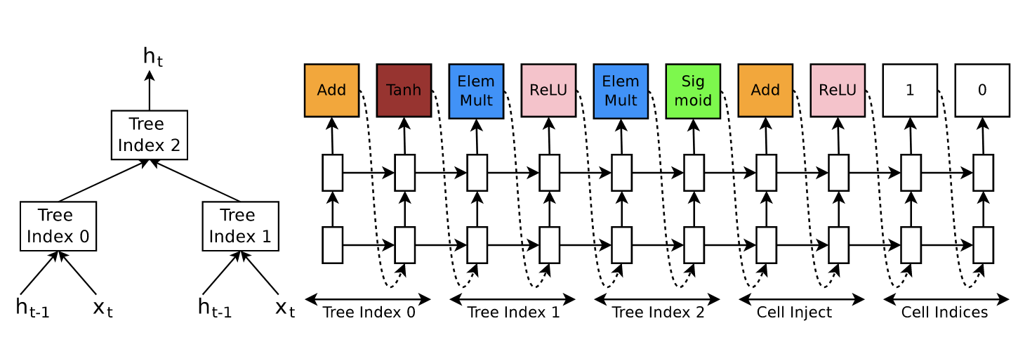
Let’s analyze it step by step. As you can see the process is split in 5. The first three are what you see, the way in which to combine $x_t$ and $h_{t-1}$ to produce $h_{t}$. However, that description is not complete because the cells state can be injected to any tree index. The last two numbers of the sequences indicate when to inject, in this example there is a 1 and a 0, which means that the cell state is injected to the tree index 0 and that the new cell state is the value in tree index 1. And the content of the cell inject part is how you inject the cell state. Let’s recap. Tree index 0 is $a_0 = \text{tanh}(W_1 \cdot x_t + W_2 \cdot h_{t-1})$, which is located at the right part of the graph above. Tree index 1 is $a_1 = \text{ReLU}(W_3 \cdot x_t \odot W_4 \cdot h_{t-1})$ located at the left. This is the simple part. Now things get complicated, the number at the end tells which tree index to inject the cell state, in this case the 0. So we have to update $a_0$ by $a_0 \leftarrow \text{ReLU}(a_0 + c_{t-1})$. Note that there are no learnable parameters in this step. Having done that we can now compute tree index 2: $a_2 = \text{sigmoid}( a_0 \odot a_{1})$. And this is the new hidden state $h_t \leftarrow a_2$. There is just one thing left, what is the new cell state? The value at tree index 1, which is the number we haven’t used yet. So the new cell state is the value at tree index 1 previous to activation so $c_t \leftarrow W_3 \cdot x_t \odot W_4 \cdot h_{t-1}$.

It is a mess at the beginning but once you understand it, is awesome. You can represent any combination by a sequence and so you can learn to generate the optimal sequence. The irony here is that we are using recurrent networks to design recurrent networks. And although the authors didn’t try it, it could be interesting to iterate that process. Use an RNN to design a better RNN, then use that new RNN to design another one and so on. My guess is that it would converge, but who knows, maybe you get an infinitely better network.

Okay, we have learned a way to represent RNN, so, how does the LSTM look like with this new representation? It looks like this

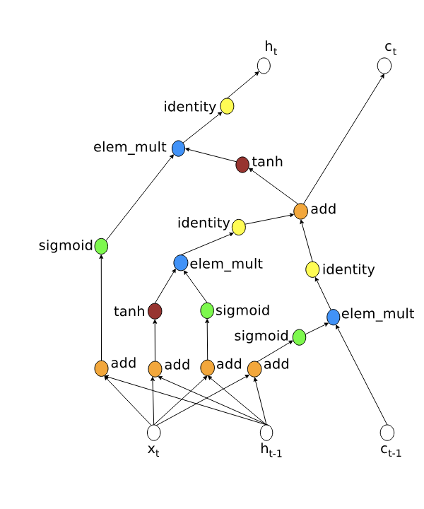
If you are interested you can go through the graph step by step to check that the formulas are the same.

Finally, the moment we were all expecting, the new and better Recurrent cell found by the authors of the NAS, the so-called NASCell (you can find it in tensorflow with that name).

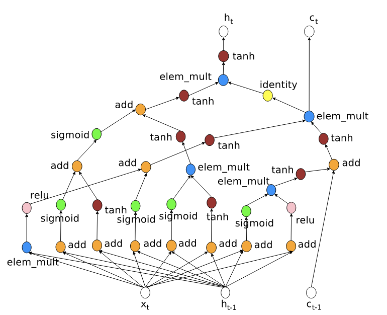
In order to find it the authors required a lot of computation. This RNN is supposed to be better at language tasks than the normal LSTM. However, since this article came before big transformers were made, this recurrent cell got forgotten after that, and didn’t get much attention. Nevertheless, it is interesting to know that there are many possible RNN, not only the LSTM and the GRU. So the next time you want to try a simple RNN instead of a big transformer, you can think of using the NASCell.

If you liked this, then you are going the enjoy the last part of this series. In the next and last chapter I will be explaining another modification of the controller to include residual connections. Making the controller capable of designing architectures such as ResNet or EfficienNet. Stay tuned!