Modelling a padel match with Hidden Markov Models (Part 2)
In my last post I explained the usefulness of Hidden Markov Models for predicting the outcome of a padel match with only a few observations. There I also showed how easy it was to implement everything in Python, but I left the most important part: the HMM itself. Today we are going to learn how to design a HMM to predict the result of a point. This is going to be an iterative process. The final model, as you will see, is a monstruosity. But step by step we are goint to build it succesfully. “Rome wasn’t made in a day”.
Inspiration and design
Before diving into the details, let me explain how I tackled this problem. I think the creative process is worth mentioning. If you just want the details, you can skip this section. Before starting to code or thinking on my own for the solution of a problem I always research for similar problems that are already solved so that I can get some inspiration. In this case, it turned out that somebody had already designed a HMM for tenis. In this article, they present a HMM for following the state of a tennis match. The observations in this article were poorly defined, but the hidden states wer very clear. I could get an idea of what I had to do by just looking at this image.
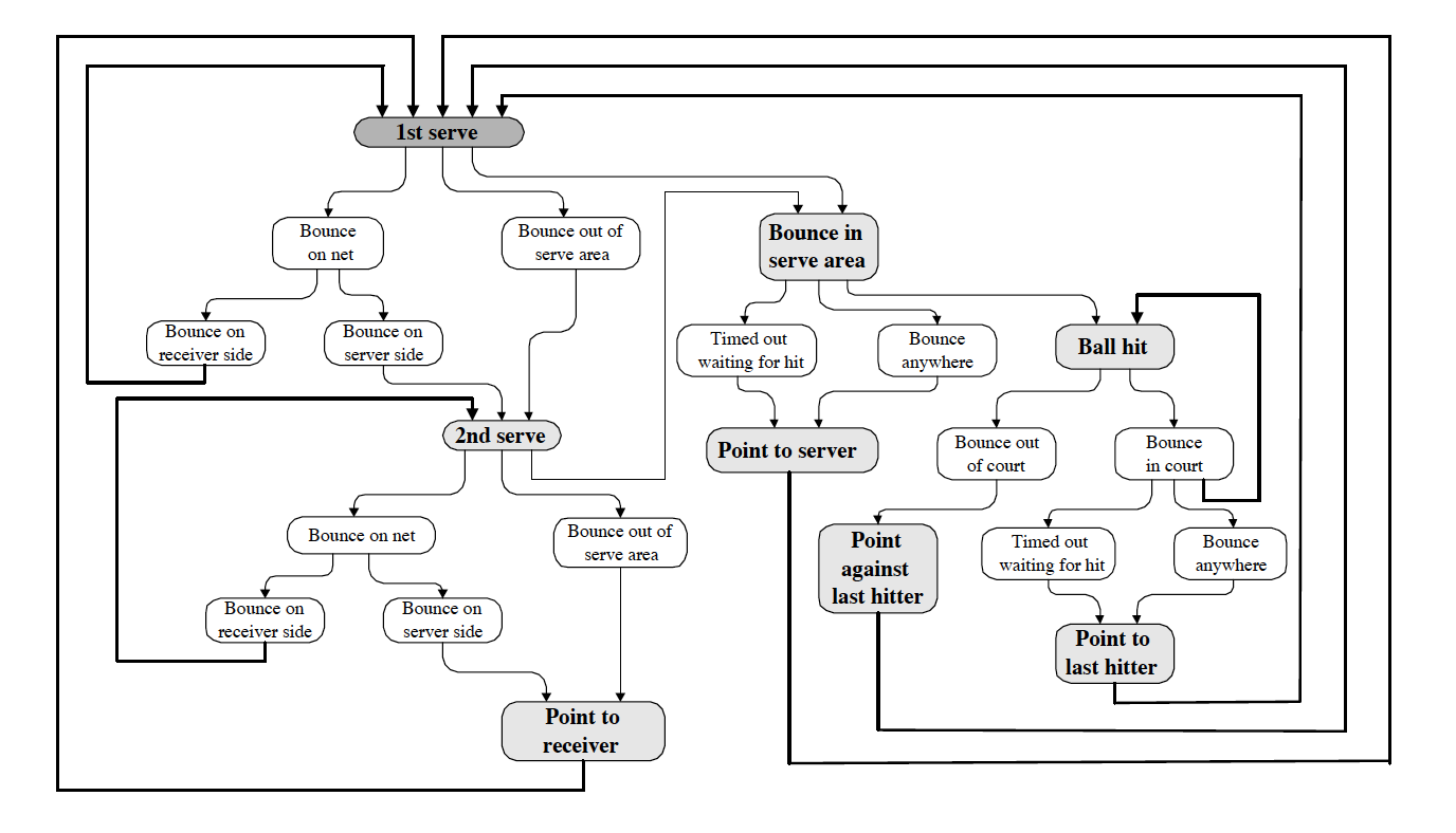
This graph is just depicting visually the rules of tenis. In our case we just have to show the rules of padel with a similar graph. If you look carefully you will see that the white boxes represent hidden states with an obvious observation. For padel there will be more of them because apart from bouncing on the ground, the ball can bounce on the walls, which makes the graph more complex but the idea is the same. Another helpful diagram on the same article represented the same graph but organised in several subgraphs.
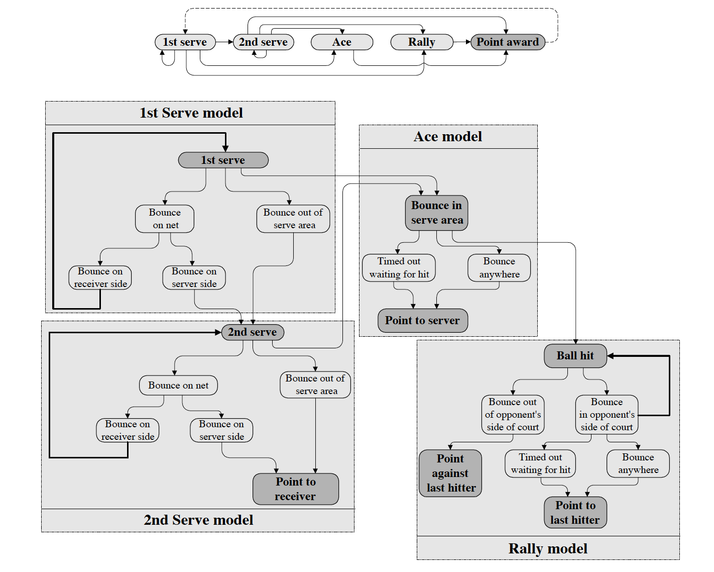
What’s interesting here is that those four subgraphs will be the same for padel. The high-level view of the process (top) is exactly the same. That’s part of the job which is already done. We just have to change the internal representation between those four subgraphs and maintain the interconnections.
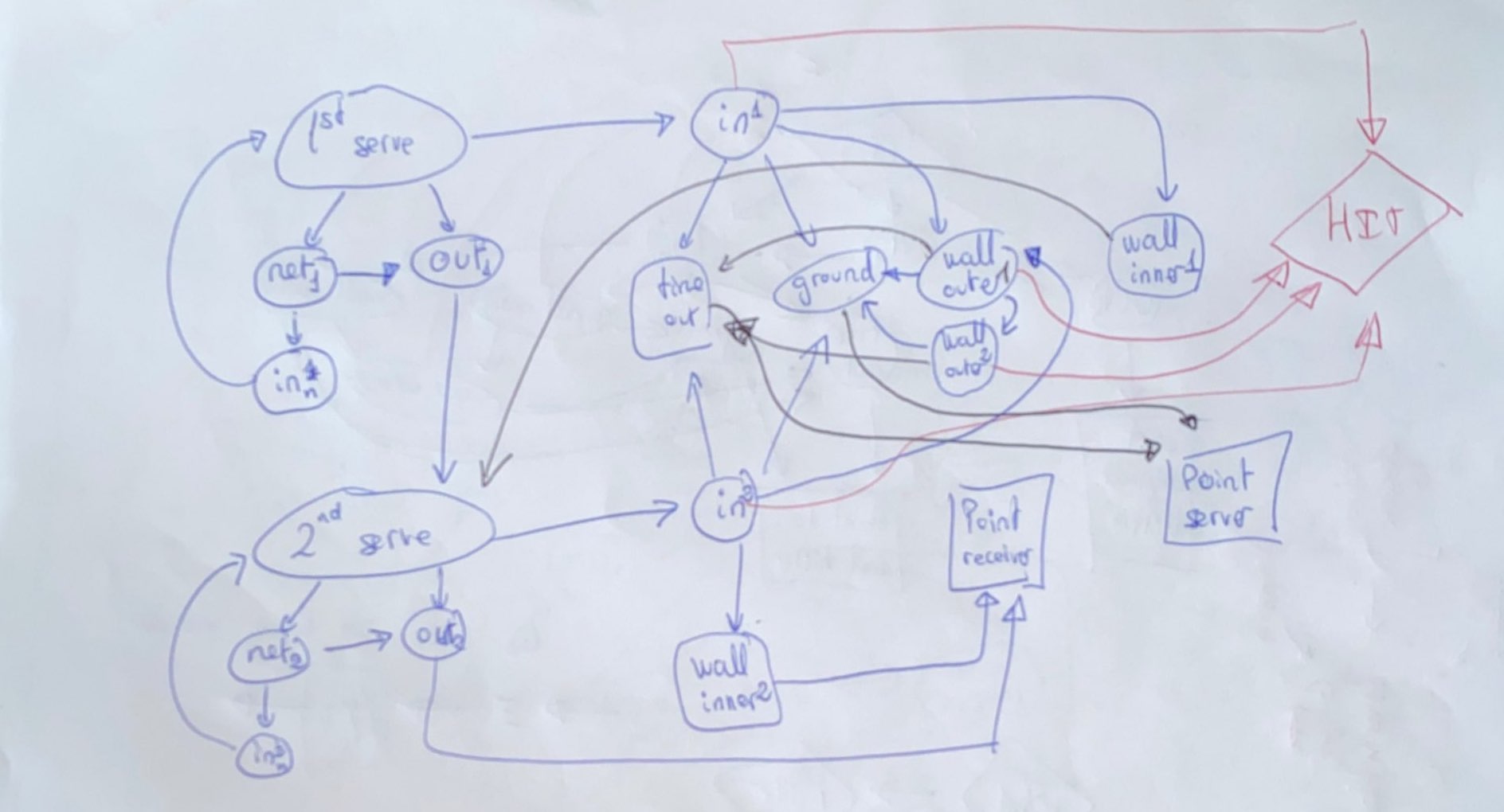
What about designing graphs? What is the software I used for that? You may say. Well, it is actually a pen and a lot of papers. No matter how well developed graph visualizations software are, drawing a simple graph by hand will always be faster than coding it. Of course, when the project keeps growing and the graphs becomes massive you will need those software tools which I will mention later. But at the beginning, just take a pen and start drawing. In the other sections I will present diagrams made with a computer because they are visually more pleasant and you will understand them better. Nevertheless, here is one of the graphs I painted by hand, in case you are curious.
The hidden states’ graph
For a HMM we need the transition and emission matrices. The transition matrix is going to be the adjacency matrix of the transitions graph. That graph is simply a representation of the rules of the game. I am going to distinguish two main parts in that rules. The rules for the serve and the rules for the normal game. The reason for creating two distinct graphs is because the effect of the ball going out or touching the net is different at the beginning.
Serve
What happens when a player is on their serve? It can go in, it can go out or it can touch the net. And if it touches the net, it can then go in or out. Let’s ignore when it goes in without touching the net for the moment. How would you represent the 1st serve? Like this?
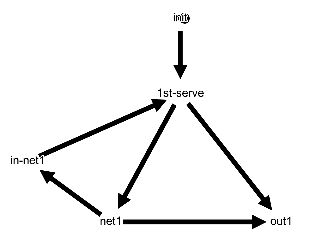
Did you think about the init state? Remember, this model is a realistic one. In practice you don’t know when is the point starting. Therefore, you need a special state for waiting until you have enough evidence that the match has begun. If you look closely, you will see that there is a self-loop on the init state. That is how we represent a waiting state in a HMM, by a self-loop. Now, let’s pass to the 2nd-serve. How would you design it?
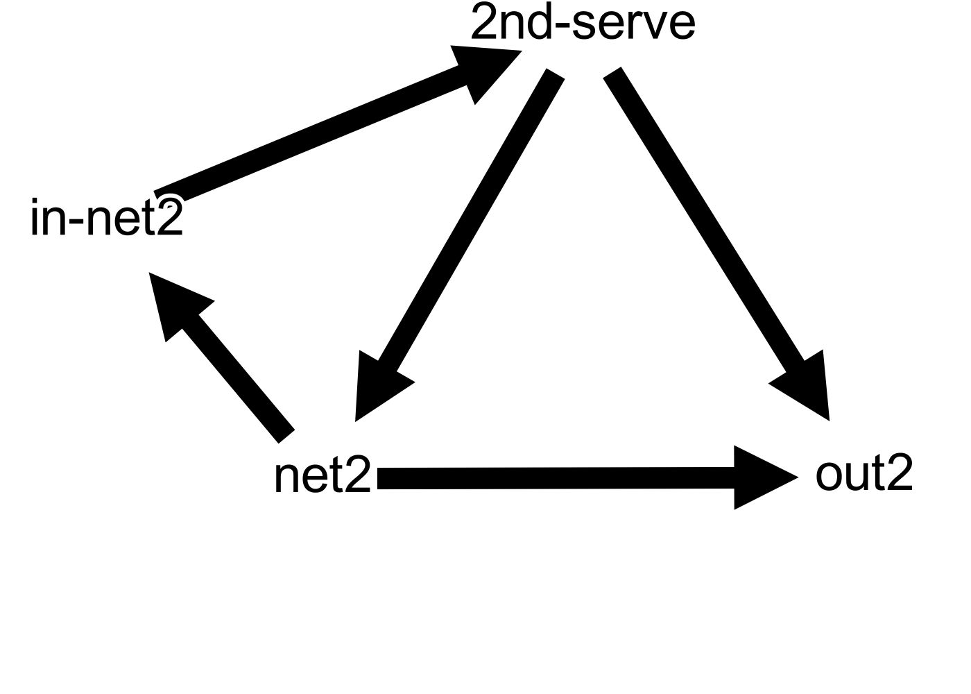
Exactly the same as the first service. The simpler, the better. We are ignoring when the ball goes in and the game continues. We are just focusing on when the ball goes out or to the net. The rest of the details will be added later on. For now let’s just focus on what we have. We have a graph with several nodes, each representing a state. What do we need? Consistent labels across the whole graph. One of the limitations of the HMM is that you have to fulfill the Markov property. Which means that the state representing going out after the 1st-serve is different than the state of going out after the 2nd-serve. So they need different names. In my case, I just added a suffix number when that happened. That way, going out in the first service is ‘out1’ and after the second is ‘out2’. Another state that repeats a lot across the graph is the ‘in’ state. For that one adding a suffix number is not enough, so I added a more descriptive suffix. For instance, going in after touching the net in the first serve is ‘in-net1’. This is a decision that could have been made of many ways, but I decided to make it like this.
Okay, let’s now talk about what happens when the ball actually goes in and the game continues. To keep it simple, let’s focus on what happens before any player hits the ball. And let’s call this the ace model. As the name states it, one of the things than can happen is an ace. What characterizes an ace? The fact that the ball touches the ground again before any player hitting it. Try to draw the scheme for the ace model. Keep in mind that before touching again the ground it can hit the walls. And also bare in mind that there are two types of walls. What are the connections among those states? Which combinations are valid and which not? Here is my solution for that problem, omitting the connections to the states Point-server and Point-receiver representing the end of the game.
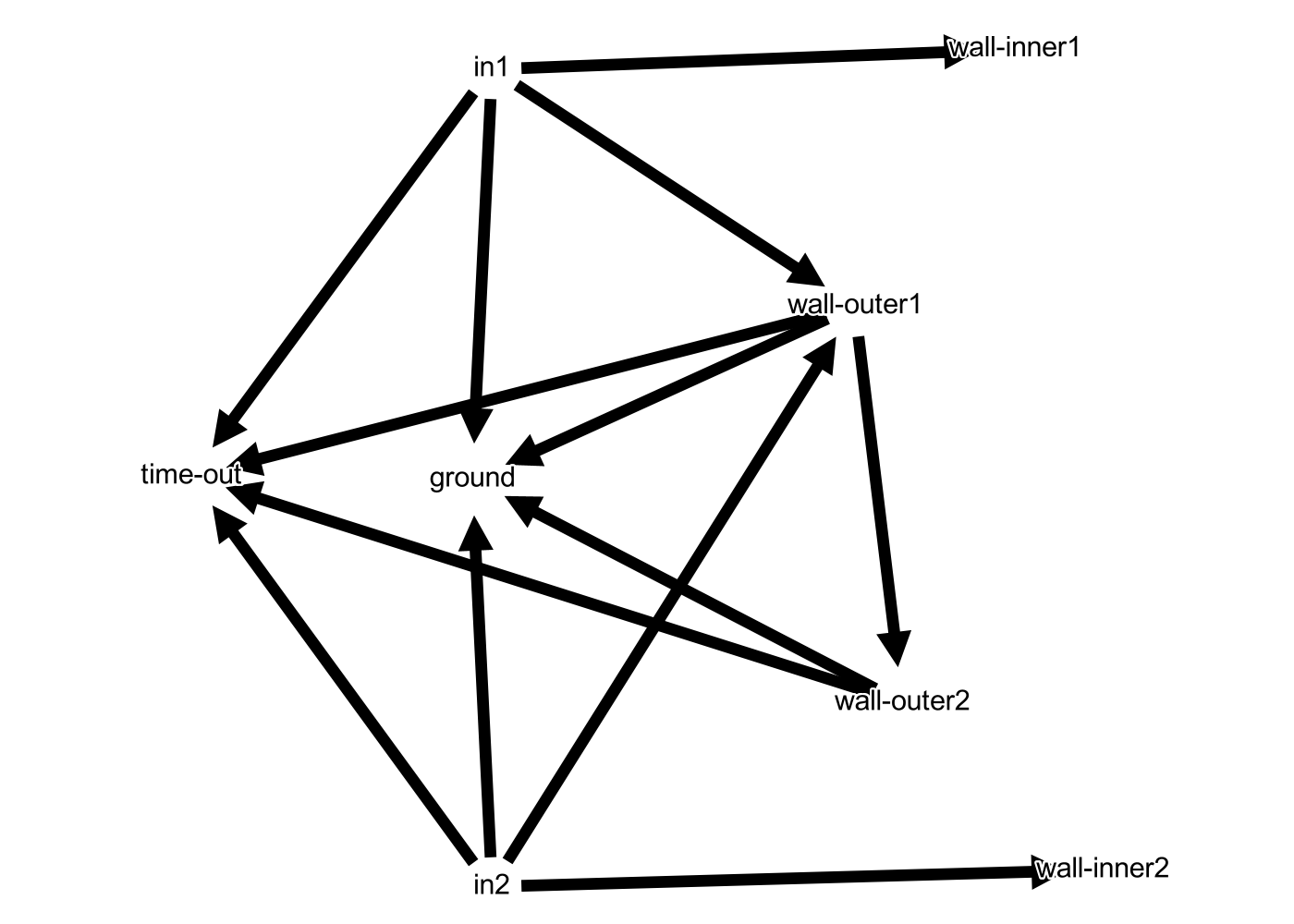
Did you thought of the ‘time-out’ state? Again, this is a real model so it has to deal with real problems. And one of them is that you miss the observation that characterizes the end of the game. If that happens you can only know the game has finished by time. That’s why you need a state to represent the end of the game by time. Later on when defining the emissions it will be made more clear why this state is needed. Most of the extra states are created so that when an observation is wrong, there is still a path in the graph to the end. Otherwise, the model will give an error and doesn’t return anything. Observe also that there are two ‘in’ states. Can you imagine why? The state ‘in1’ is when the ball goes in on the first serve, and ‘in2’ on the second. Since we have to maintain the Markov property, those two states are different although they have the same emissions and are identical to us.
Before going to the next block, which is when a player hits the ball and the game actually starts, let me explain how I made this pictures and how you can code graphs on Python. With the library networkx you can do many thing on graphs, it has implemented almost every algorithm that exists related to graphs. In this project we only use it to define the graphs. The syntax is pretty straighforward, you define a DiGraph which stands for directed graph, and add nodes and edges with the functions add_nodes_from and add_edges_from. After that, you can save the model in gml format and open it with Gephi. That’s it. Here is the code for the three models presented above.
1
2
3
4
5
6
7
8
9
10
11
12
13
14
15
16
17
18
19
20
21
22
23
24
25
26
27
28
29
30
31
32
33
34
35
36
37
38
39
40
41
42
43
44
45
46
47
48
49
50
51
52
53
54
55
import networkx as nx

folder_path = 'graphs/'

""" First serve model """
first = nx.DiGraph()
first.add_nodes_from([
    ("init", {"hidden": True}),
    ("1st-serve", {"hidden": True}),
    ("net1", {"hidden": True}),
    ("out1", {"hidden": True}),
    ("in-net1", {"hidden": True}),
])
first.add_edges_from([
    ("init", "1st-serve"), ("init", "init"),
    ("1st-serve","net1"), ("1st-serve","out1"),
    ("net1","in-net1"), ("net1","out1"),
    ("in-net1","1st-serve")
])
nx.write_gml(first, folder_path + 'first.gml')

""" Second serve model """
second = nx.DiGraph()
second.add_nodes_from([
    ("2nd-serve", {"hidden": True}),
    ("net2", {"hidden": True}),
    ("out2", {"hidden": True}),
    ("in-net2", {"hidden": True}),
])
second.add_edges_from([
    ("2nd-serve","net2"), ("2nd-serve","out2"),
    ("net2","in-net2"), ("net2","out2"),
    ("in-net2","2nd-serve")
])
nx.write_gml(second, folder_path + 'second.gml')

""" Ace model """
ace = nx.DiGraph()
ace.add_nodes_from([
    ("in1", {"hidden": True}),
    ("in2", {"hidden": True}),
    ("time-out", {"hidden": True}),
    ("ground", {"hidden": True}),
    ("wall-outer1", {"hidden": True}),
    ("wall-outer2", {"hidden": True}),
    ("wall-inner1", {"hidden": True}),
    ("wall-inner2", {"hidden": True}),
])
ace.add_edges_from([
    ("in1", "time-out"), ("in1", "ground"), ("in1", "wall-outer1"), ("in1", "wall-inner1"),
    ("in2", "time-out"), ("in2", "ground"), ("in2", "wall-outer1"), ("in2", "wall-inner2"),
    ("wall-outer1", "time-out"), ("wall-outer1", "ground"), ("wall-outer1", "wall-outer2"),
    ("wall-outer2", "time-out"), ("wall-outer2", "ground"),
])
nx.write_gml(ace, folder_path + "ace.gml")
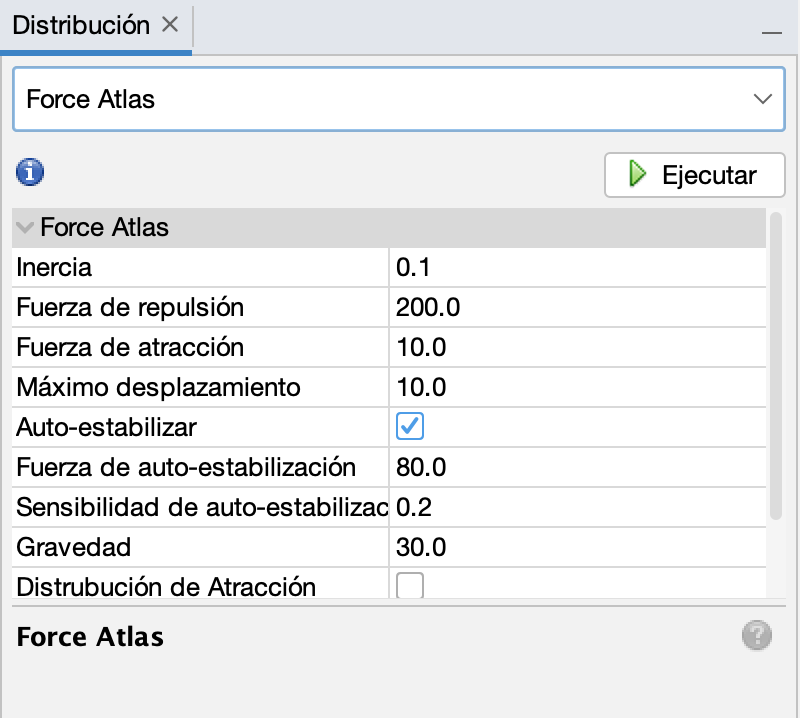
Gephi has some handy features that make posible visualize big graphs. Concretely, you can use the Force Atlas distribution to reorder the nodes by simulating forces proportional to the number of edges they have. It has many parameters you can try, but I normally just click on execute and wait a few seconds for convergence.
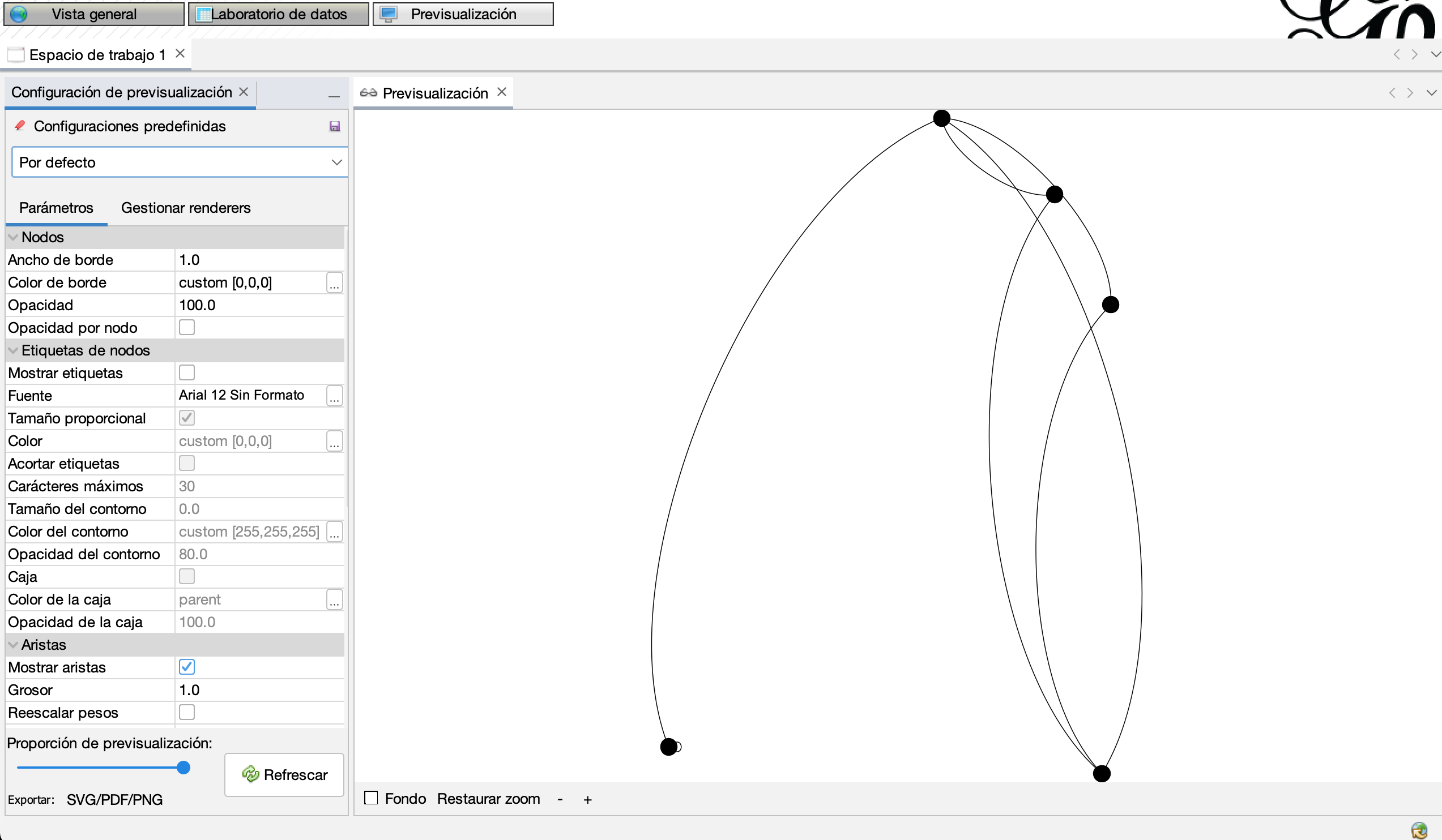
Then, on the previsualization tab, you can create the diagrams I showed you. It has many options, like curved edges. I don’t use that feature for this post because for complex graphs it can be messy. But for some graphs I think is prettier with curvy edges. Other things to adapt are the font size and the size of the arrows. With a bit of practice you can create nice figures quite fast.
Rally
The rally model is a bit more complex than the ones presented above. There are two ways to design it based on which observations you have. If you only have an observation for bouncing on the ground, anywhere, then the rally model only has one ‘HIT’ state and the rest is similar to the ace model. However, in practice you can have more information than that. Suppose you have an image of a game and you know the location of the ball together with the fact that it is a bounce in the ground. You could, potentially, distinguish if the ball is on the server side or on the receiver side. You just need to segment the court and see if the ball is on the upper side or not. This is not trivial, but is possible to achieve. For that reason, we are going to have two ‘HIT’ states: one for the server side and one for the receiver. The rest is just identical to the ace model, with one exception. Instead of ending the game or returning to the beginning, the states point to the other ‘HIT’ states. Similar to what would happen in a match. Your head is going from one side to the other. Here the hidden state is moving from one model to the other. Finally, the diagram.
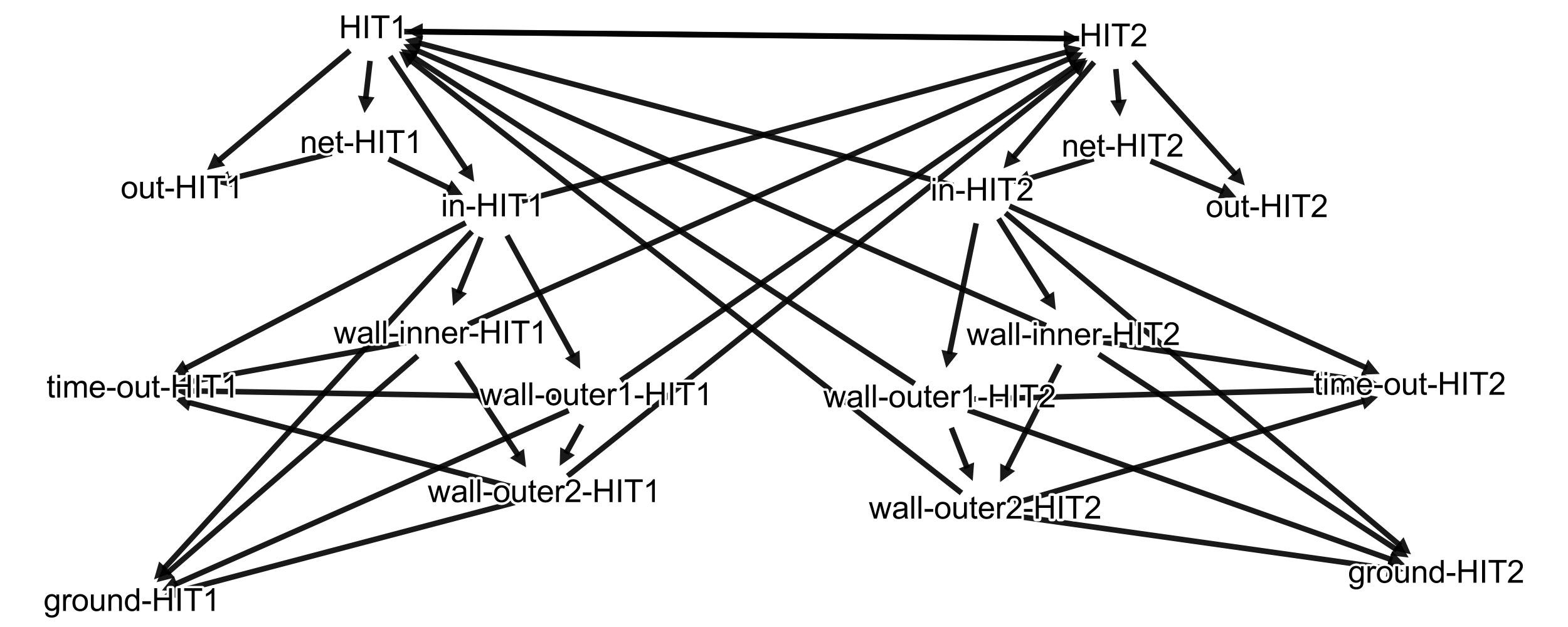
If you understood the ace model, you just need to focus on the arrows that cross from left to right and vice versa. The rest is just the standard mechanics of a padel game. One more thing to notice is that there are many arrows missing. Concretely, the arrow between the models and the arrows that point to the absorbing states, that is, those which end the game. In the next section, I will try to describe the connections between the models and will show you the (almost) full picture of the HMM transition graph. Also, below is the code for this model.
1
2
3
4
5
6
7
8
9
10
11
12
13
14
15
16
17
18
19
20
21
22
23
24
25
26
27
28
29
30
31
32
33
34
35
36
37
38
39
40
41
42
43
44
""" Rally model """
rally = nx.DiGraph()
rally.add_nodes_from([
    ("HIT1", {"hidden": True}),
    ("net-HIT1", {"hidden": True}),
    ("in-HIT1", {"hidden": True}),
    ("out-HIT1", {"hidden": True}),
    ("time-out-HIT1", {"hidden": True}),
    ("ground-HIT1", {"hidden": True}),
    ("wall-inner-HIT1", {"hidden": True}),
    ("wall-outer1-HIT1", {"hidden": True}),
    ("wall-outer2-HIT1", {"hidden": True}),

    ("HIT2", {"hidden": True}),
    ("net-HIT2", {"hidden": True}),
    ("in-HIT2", {"hidden": True}),
    ("out-HIT2", {"hidden": True}),
    ("time-out-HIT2", {"hidden": True}),
    ("ground-HIT2", {"hidden": True}),
    ("wall-inner-HIT2", {"hidden": True}),
    ("wall-outer1-HIT2", {"hidden": True}),
    ("wall-outer2-HIT2", {"hidden": True}),
])
rally.add_edges_from([
    ("HIT1", "out-HIT1"), ("HIT1", "in-HIT1"), ("HIT1", "net-HIT1"),
    ("in-HIT1", "HIT2"), ("wall-inner-HIT1", "HIT2"), ("wall-outer1-HIT1", "HIT2"), ("wall-outer2-HIT1", "HIT2"),
    ("net-HIT1", "in-HIT1"), ("net-HIT1", "out-HIT1"),
    ("in-HIT1", "time-out-HIT1"), ("in-HIT1", "ground-HIT1"), ("in-HIT1", "wall-inner-HIT1"), ("in-HIT1", "wall-outer1-HIT1"),
    ("wall-inner-HIT1", "time-out-HIT1"), ("wall-inner-HIT1", "ground-HIT1"), ("wall-inner-HIT1", "wall-outer2-HIT1"),
    ("wall-outer1-HIT1", "time-out-HIT1"), ("wall-outer1-HIT1", "ground-HIT1"), ("wall-outer1-HIT1", "wall-outer2-HIT1"),
    ("wall-outer2-HIT1", "time-out-HIT1"), ("wall-outer2-HIT1", "ground-HIT1"),

    ("HIT1", "HIT2"), ("HIT2", "HIT1"),

    ("HIT2", "out-HIT2"), ("HIT2", "in-HIT2"), ("HIT2", "net-HIT2"),
    ("in-HIT2", "HIT1"), ("wall-inner-HIT2", "HIT1"), ("wall-outer1-HIT2", "HIT1"), ("wall-outer2-HIT2", "HIT1"),
    ("net-HIT2", "in-HIT2"), ("net-HIT2", "out-HIT2"),
    ("in-HIT2", "time-out-HIT2"), ("in-HIT2", "ground-HIT2"), ("in-HIT2", "wall-inner-HIT2"), ("in-HIT2", "wall-outer1-HIT2"),
    ("wall-inner-HIT2", "time-out-HIT2"), ("wall-inner-HIT2", "ground-HIT2"), ("wall-inner-HIT2", "wall-outer2-HIT2"),
    ("wall-outer1-HIT2", "time-out-HIT2"), ("wall-outer1-HIT2", "ground-HIT2"), ("wall-outer1-HIT2", "wall-outer2-HIT2"),
    ("wall-outer2-HIT2", "time-out-HIT2"), ("wall-outer2-HIT2", "ground-HIT2")

])
nx.write_gml(rally, folder_path + "rally.gml")
Interconnections
Let’s go model by model, edge by edge, starting by the 1st-serve. It has two connections, one to the ‘in1’ state of the ace model and one to the 2nd-serve. The latter is from the ‘out1’ state, if the ball goes out, you have a second service, that’s the rules. The 2nd-serve model is similar, one connection to the ‘in2’ state and one to the absorbing state ‘Point-receiver’. If you fail your second serve, you lose the point. Simple, concise and clear. Let’s continue with the ace model. The ‘ground’ and ‘time-out’ states point to ‘Point-server’. This is the representation of an ace. If the ball hits the ground twice, it’s an ace and the point goes to the server side. The rest of the connections are to the ‘HIT1’ state, which means that the receiver has hit the ball and the game continues. And that’s it. The only remaining connections are between the rally model and the absorbing states, just like in the ace model. If the ball bounces twice, or if it goes out of the court after bouncing in, the last player wins. If it goes out, the last player loses. For those of you that know how to play padel, this should be no surprise. There are many cases to deal with because the ball can hit the walls and the net. But more or less it is summarized like that. Here’s the full picture.
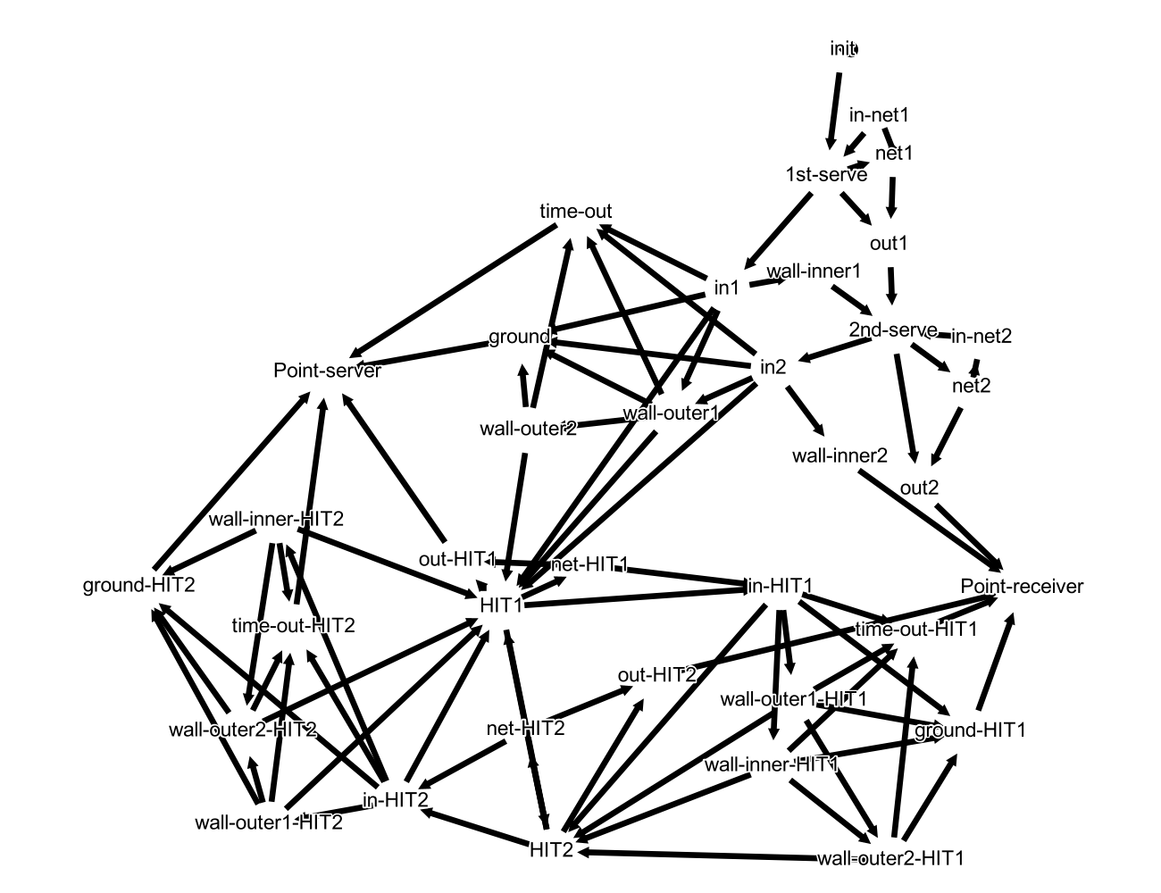
The code for this part is different. This time we have to join the four different models. To do so we are going to use the function union_all that creates a new graph with all the nodes and edges from before but without any connections between the subgraphs. To add those connections we use the add_edge function and for the absorbing states the add_nodes_from. This is the result.
1
2
3
4
5
6
7
8
9
10
11
12
13
14
15
16
17
18
19
20
21
22
23
24
25
26
27
28
29
""" Graph union plus connection edges """
union = nx.union_all((first, second, ace, rally))
union.add_edge("out1", "2nd-serve")
union.add_edge("1st-serve", "in1")
union.add_edge("2nd-serve", "in2")
union.add_edge("wall-inner1", "2nd-serve")

""" Absorbing states """
union.add_nodes_from([
    ("Point-receiver", {"hidden": True}),
    ("Point-server", {"hidden": True})
])
union.add_edge("wall-inner2", "Point-receiver")
union.add_edge("out2", "Point-receiver")
union.add_edge("time-out", "Point-server")
union.add_edge("ground", "Point-server")
union.add_edge("out-HIT1", "Point-server")
union.add_edge("time-out-HIT1", "Point-receiver")
union.add_edge("ground-HIT1", "Point-receiver")
union.add_edge("out-HIT2", "Point-receiver")
union.add_edge("time-out-HIT2", "Point-server")
union.add_edge("ground-HIT2", "Point-server")

""" Connection between ace and rally """
union.add_edge("in1", "HIT1")
union.add_edge("in2", "HIT1")
union.add_edge("wall-outer1", "HIT1")
union.add_edge("wall-outer2", "HIT1")
nx.write_gml(union, folder_path + "union.gml")
Delays
Previously I said this was almost the full picture. The reason for that is that the model here does not take into account that the ball is flying in between bounces. In an ideal model this would be irrelevant, with just the bounces we can predict the outcome of the game. But in practice that is not true. Do you remember the reason for using a ‘time-out’ state? Here is similar. Imagine you detect the same bounce twice by error. If you only look at bounces you will assume that the game has finished. However, if you detect twice the same bounce, in time they will be very close. In contrast with what will happen if those two bounces are both real. Therefore, if you somehow take into account the time between observations you can solve those kind of errors. The way to do that is by adding ‘flying’ states. In between any two states you include a ‘flying’ state and in the emissions you consider ‘flying’ as a plausible observation. This way you have a way of measuring time. The more ‘flying’ observations you have, the more time that has passed between states. The key here is that the ‘flying’ state has a self-loop. Similar to the ‘init’ state. You don’t know how much time is going to occur between states. For that reason you add a self-loop to stay in that state until there is evidence enough that you are not flying anymore.
For this part there is no diagram. As you may have guessed, adding one state for every edge is going to make the model huge and very complicated to deal with. At this step, I mostly work with the code. Adding all the edges by hand is a nightmare. For that reason, I let python do that for me. Before showing you the code, there is one more hypothesis to deal with. I said that the reason for the ‘flying’ state is to correct duplicate observations. But to do that it is needed to add more than one ‘flying’ state per edge. Why? Because the first ‘flying’ states are going to be corrective states without self-loop. It is only the last one that is a waiting state. Those corrective states can emit the same observations as the first state. While the waiting state can only emit the ‘flying’ observation. The reason for this is mostly empirical. Using only one ‘flying’ state yielded unsatisfactory results. In my experiments I ended up using five ‘flying’ states: four correctives, and one waiting. Finally, the code for that.
1
2
3
4
5
6
7
8
9
10
11
12
13
14
15
""" Add flying states """
current_edges = list(union.edges)
fly_err_len = 5
for (u,v) in current_edges:
    if u == "init":
        continue
    union.add_nodes_from([("flying-"+u+'-'+str(k), {"hidden": True}) for k in range(fly_err_len+1)])
    union.remove_edge(u, v)
    union.add_edge(u, "flying-"+u+"-0")
    union.add_edge(u, "flying-"+u+"-"+str(fly_err_len))
    for k in range(fly_err_len):
        union.add_edge("flying-"+u+'-'+str(k), "flying-"+u+'-'+str(k+1))
        union.add_edge("flying-"+u+'-'+str(k), "flying-"+u+'-'+str(fly_err_len))
    union.add_edge("flying-"+u+'-'+str(fly_err_len), "flying-"+u+'-'+str(fly_err_len))
    union.add_edge("flying-"+u+'-'+str(fly_err_len), v)
And the last part of the code is to convert the ‘Point-server’ and ‘Point-receiver’ states into waiting states. The reason for this is numerical. When creating the transition and emission matrices the values need to be normalized. If you don’t add this connections you have rows with all zeros that give errors and it is easier to solve them like this. Those edges are added after creating the ‘flying’ states because those edges don’t need any ‘flying’ states attached to them, they are simply a trick for the computation.
1
2
3
""" Self-loops for absorbing states """
union.add_edge("Point-receiver", "Point-receiver")
union.add_edge("Point-server", "Point-server")
The observations’ graph
First, let’s define the observations.
1
2
3
4
5
6
7
8
9
10
11
12
""" Possible observations """
obs = nx.DiGraph()
obs.add_nodes_from([
    ("player-hit", {"hidden": False}),
    ("bounce-ground-receiver", {"hidden": False}),
    ("bounce-ground-server", {"hidden": False}),
    ("bounce-net", {"hidden": False}),
    ("bounce-wall-inner", {"hidden": False}),
    ("bounce-wall-outer", {"hidden": False}),
    ("flying", {"hidden": False}),
    ("end", {"hidden": False})
])
This is all we can observe, at least automatically with a camera. We can observe the ball bouncing anywhere: in the walls, in the net, or in the ground. And we can observe any player hitting the ball. Notice that we don’t have to distinguish which player hits the ball, that job is done by distinguishing where is the ball bouncing. The reason for that is that it is quite difficult in practice to detect when a player hits the ball and which player it is due to projection. With just one observation representing all the player is enough to solve the problem. Keep in mind that this is for real cases, and the model has to reflect the limitations of the detections. There is one special observation called ‘end’. The HMM presented here can only deal with isolated points. The ‘end’ observation is only emitted by the absorbing states. It is a way of forcing the HMM to find a solution. When dealing with more than one point it is needed to detect when the point has finished.
As with the ‘flying’ states, I didn’t add all the emissions by hand. There are a lot of nodes in the transition graph. And the emission graph is a bipartite graph with transitions on one side and emissions on the other. That is a lot of edges. But in the end, is no more than a regex problem. The states have descriptive names. Any state with ‘ground’ in their name is going to emit either ‘bounce-ground-receiver’ or ‘bounce-ground-server’. And the ‘flying’ states emit the ‘flying’ observation. There is no fancy ideas here, just nasty work. I leave here the code for you. There are better ways to code this for sure, but this works and it’s mine, so I like it.
There are two more things to mention. The flying probability and the missing probability. As I said before there are corrective states. Those corrective states can emit the same observation as the state they are attached to it, but with a smaller probability. Otherwise, if the probability isn’t lower, we are not taking into account the fact that the more separated two observations are, the more likely they are to be correct. Thus, the corrective ‘flying’ states have some probability of emit ‘flying’ and some probability of emiting other things. The missing probability is similar but is for the other states. If instead of a duplicate you miss an observation, the graph still needs to find a path to the end. For that reason every state has some little probability of emitting ‘flying’. And there are many other little changes that were added in the process of creating this matrix. The justification behind most of the strange things you will see in the code is empirical. You start with a simple model and find a case where it doesn’t work, change the model and repeat. After several iterations you arrive at this.
1
2
3
4
5
6
7
8
9
10
11
12
13
14
15
16
17
18
19
20
21
22
23
24
25
26
27
28
29
30
31
32
33
34
35
36
37
38
39
40
41
42
43
44
45
46
47
48
49
50
51
52
53
54
55
56
57
58
59
60
61
62
63
64
65
66
67
68
69
70
71
72
73
74
75
76
""" Create bipartite graph representing emissions """
G = union.copy()
G.clear_edges()
U = nx.union(G, obs)
flying_prob = 0.9
err_miss_prob = 0.001
eps = 1e-12
for u in G.nodes():
    if "Point" in u:
        #U.add_weighted_edges_from([(u, "flying", 1)])
        U.add_weighted_edges_from([(u, "end", 1)])
        continue
    if "flying" in u and "init" not in u:
        U.add_weighted_edges_from([(u, "flying", flying_prob)])
        U.add_weighted_edges_from([(u, "bounce-ground-server", eps)])
        U.add_weighted_edges_from([(u, "bounce-ground-receiver", eps)])
        if fly_err_len > 0 and fly_err_len == int(u.split('-')[-1]):
            continue
    elif u not in ["net1", "net2", "wall-inner1", "wall-inner2"]:
        U.add_weighted_edges_from([(u, "flying", err_miss_prob)])

    if "init" in u:
        U.add_weighted_edges_from([(u, "bounce-ground-receiver", (1-flying_prob)/5)])
        U.add_weighted_edges_from([(u, "bounce-ground-server", (1-flying_prob)/5)])
        U.add_weighted_edges_from([(u, "bounce-wall-inner", (1-flying_prob)/5)])
        U.add_weighted_edges_from([(u, "bounce-wall-outer", (1-flying_prob)/5)])
        U.add_weighted_edges_from([(u, "bounce-net", (1-flying_prob)/5)])
        # U.add_weighted_edges_from([(u, "player-hit", eps)])
        U.add_weighted_edges_from([(u, "flying", flying_prob)])
    elif "serve" in u or u == "HIT1" or u == "HIT2" or "flying-HIT1-" in u or "flying-HIT2-" in u:
        U.add_weighted_edges_from([(u, "player-hit", 1-flying_prob)])
        U.add_weighted_edges_from([(u, "bounce-ground-receiver", eps)])
        U.add_weighted_edges_from([(u, "bounce-ground-server", eps)])
        U.add_weighted_edges_from([(u, "bounce-wall-inner", eps)])
        U.add_weighted_edges_from([(u, "bounce-wall-outer", eps)])
    elif "time" in u:
        U.add_weighted_edges_from([(u, "flying", 1)])
    elif "wall" in u: # this must be before in and out
        if "inner" in u:
            U.add_weighted_edges_from([(u, "bounce-wall-inner", 1-flying_prob)])
        elif "outer" in u:
            U.add_weighted_edges_from([(u, "bounce-wall-outer", (1-flying_prob)/2)])
            if "HIT1" in u:
                U.add_weighted_edges_from([(u, "bounce-ground-server", (1-flying_prob)/2)])
            elif "HIT2" in u:
                U.add_weighted_edges_from([(u, "bounce-ground-receiver", (1-flying_prob)/2)])
        else: assert(False)
        U.add_weighted_edges_from([(u, "player-hit", eps)])
    elif ("in" in u or "ground" in u) and "flying-net" not in u and "flying-out" not in u:
        if "in1" in u or "in2" in u or "in-HIT2" in u or "ground-HIT2" in u\
            or "in-net1" in u or "in-net2" in u:
            U.add_weighted_edges_from([(u, "bounce-ground-receiver", 1-flying_prob)])
            if "ground-HIT2" in u:
                U.add_weighted_edges_from([(u, "bounce-ground-server", eps)])
        elif "in-HIT1" in u or "ground-HIT1" in u:
            U.add_weighted_edges_from([(u, "bounce-ground-server", 1-flying_prob)])
            if "ground-HIT1" in u:
                U.add_weighted_edges_from([(u, "bounce-ground-receiver", eps)])
        elif "ground" in u:
            U.add_weighted_edges_from([(u, "bounce-ground-receiver", 1-flying_prob)])
            U.add_weighted_edges_from([(u, "bounce-ground-server", eps)])
        else: assert(False)
        U.add_weighted_edges_from([(u, "player-hit", eps)])
    elif "out" in u:
        if "out-HIT1" in u:
            U.add_weighted_edges_from([(u, "bounce-ground-receiver", (1-flying_prob) / 4)])
        elif "out-HIT2" in u or "out1" in u or "out2" in u:
            U.add_weighted_edges_from([(u, "bounce-ground-server", (1-flying_prob) / 4)])
        U.add_weighted_edges_from([(u, "bounce-wall-inner", (1-flying_prob) / 4)])
        U.add_weighted_edges_from([(u, "bounce-wall-outer", (1-flying_prob) / 4)])
        U.add_weighted_edges_from([(u, "bounce-net", (1-flying_prob) / 4)])
        U.add_weighted_edges_from([(u, "player-hit", eps)])
    elif "net" in u:
        U.add_weighted_edges_from([(u, "bounce-net", 1-flying_prob)])
        #U.add_weighted_edges_from([(u, "player-hit", eps)])
The matrices
Okay, we have the graphs, but what about the matrices? We need those for the hmmkay library. How do we generate them? NetworkX provides a function for generating adjacency matrices (adjacency_matrix). However, we cannot use those matrices as they are, we need to normalize them so that the rows sum up to one. Remember, they represent probabilities. After normalization, we can save the result using pandas.
1
2
3
4
5
6
7
8
9
10
11
12
13
14
15
16
import pandas as pd

""" Emission matrix """
V1 = len(G.nodes())
B = nx.adjacency_matrix(U).toarray()[:V1,V1:]
err_change = 0
B += err_change
B = B / B.sum(axis=1).reshape((-1,1))
B_df = pd.DataFrame(B, columns=obs.nodes(), index=G.nodes())
B_df.to_csv(folder_path + 'B.csv')

""" Transition matrix """
A = nx.adjacency_matrix(union).toarray()
A = A / A.sum(axis=1).reshape((-1,1))
A_df = pd.DataFrame(A, columns=G.nodes(), index=G.nodes())
A_df.to_csv(folder_path + 'A.csv')
The err_change variable is for adding noise to the emissions so that every state can emit every observation with a little probability. In my experience it doesn’t work well, but I leave it there in case you want to experiment with it.
Conclusion
In this post we have seen how to properly design a HMM for following the result of a padel match. We have learnt to use the NetworkX library to create the graphs and the Gephi program to visualize the process. In the next post of this series we will learn how to actually test whether the HMM works. Stay tuned.