The so-called Generative Adversarial Networks have been with us since 2014, producing amazing results lately. Today I am bringing the proof of why they work. That is, a proof that states GANs are optimal in the limit when no parametric model is taken into account. But first, what is a GAN and what “amazing results” am I talking about?

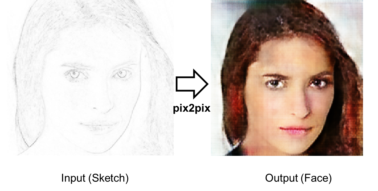
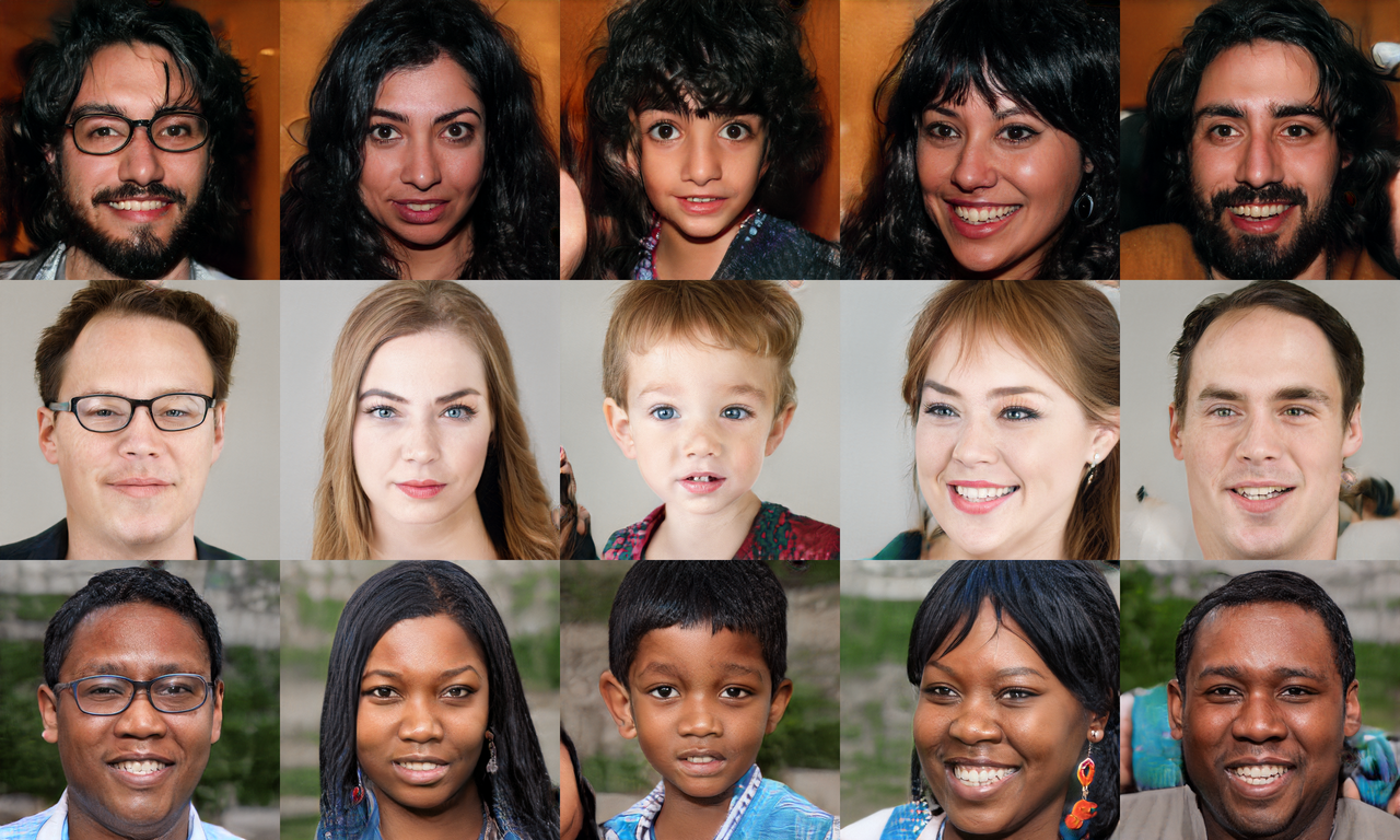
The above example is about pix2pix which is a conditional adversarial network which gives style to your draft. You draw some sketch, tell some style and the network does the rest of the work. But there are other types of GANs, like style GAN which is very good at generating images of some given type, like the ones below, which are all artificial.

GANs are also related to DALLE-2, the famous text-to-image model. Both are a special case of energy-based models, which is a more general framework. If you want to know more about it you can look at the Yann Lecunn lectures about it.

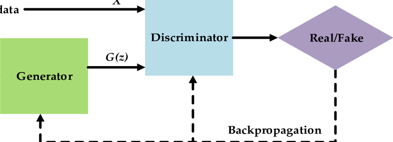
Let’s dive into the details of the original GAN formulation. Typically, GANs are presented with the following diagram.

But I prefer to understand models in the mathematical realm. There a GAN is a min-max problem. Concretely it is this min-max problem:

Where $D$ is the discriminator, it receives an image an outputs the probability of it being fake. $G$ is the generator, it receives some input vector $\textbf{z}$ and outputs a fake image, denoted by $\textbf{x}$. $V$ is a value function, which is defined as follows (each term will be explained in detail later):

How can we interpret those two terms? The first one is large when the discriminator is correctly identifying real images as real. The second one is large when the discriminator is correctly identifying the generator images as fake. Maximising this quantity yields a perfect discriminator. However, we want more than that, we want to fool the discriminator. That means creating a good generator. Fooling the discriminator means minimising the value function. Thus, we have the min-max problem as stated above. Intuitively the equilibrium of this problem will be reached when we have a perfect generator and the discriminator always outputs $\frac{1}{2}$ because the generated images are the same as the real ones. This is exactly what the optimality theorem from the original Ian Goodfellow’s paper proves.

To understand the theorem, it is needed to give some formalism to the intuitive idea of perfect generator. What is a perfect generator? For us humans, it means that the images seem real. But mathematically, what does “real” means? It means that the probability distribution of the generated images and the probability distribution of the data are the same. Mathematically the images are random variables, whose observations are represented by a vector. If the real and fake vectors come from the same distribution, then, they can be considered to be the same. As an example, consider the probability distribution function (pdf) of images of Granada. From that pdf it is more probable to draw an image of the Alhambra than an image of the Eiffel tower. Also, random noise has zero probability on that pdf. So now, a good generator pdf should mimick that behaviour, giving high probability to images of Granada and low probability to everything else.

In mathematical terms, the data pdf is denoted by $p_{data}(\textbf{x})$ and the generator pdf is $p_{g}(\textbf{x})$. So producing “real” images means that $p_{data}(\textbf{x}) = p_{g}(\textbf{x})$, $\forall \textbf{x}$. Now we can state the optimality theorem:

Before proving it, let’s analyse the consequences of it and what it is telling us. The main takeaway is that the solution to the min-max problem gives a perfect generator, which means that we can learn to reproduce any probability distribution. For simpler distributions this doesn’t seem much, one can simply compute the histogram of a variable and use it as the estimated distribution. However, for images that is not possible. How can you compute the histogram of a set of images? There are no repeated values, we just have a bunch of different images with some similarities. So one can think of a GAN as a way of estimating the histogram of a set of images. But it is more than that, it also provides a way of drawing points (images) from that distribution.

Another takeaway from the theorem is the optimal value of the value function. It may seem useless at first but it is a good indicator of whether or not the training is converging or not. Because in practice that optimal generator does not appears to us by divine revelation, an iterative method is typically used to find it. If you see that during training the model converges to a value different than $-\log(4) \approx -1.38$ then you can be certain that you have not solved the min-max problem.

So far so good but, the generator as presented above is just a deterministic function, where does the variability comes from? It is there on the formulas, you just need to give a closer look. When defining the value function the second term was computed from the distribution $p_{\textbf{z}}$, what is that? It is a prior distribution for the input of the generator, which means that the generator is a function transforming one distribution into another. Mathematically this means $\textbf{z} \sim p_{\textbf{z}} \Rightarrow G(\textbf{z}) \sim p_g$, a key fact that will be used in the proof. The inference process is now quite easy, just draw a point from $p_{\textbf{z}}$ and apply the generator to get a new image. In practice you can just put any value you want for $\textbf{z}$ since the prior is a noise prior, not anything in particular.

Finally, let’s prove the theorem. The first step is to find the optimal discriminator given the generator. After that, that value is substituted into the formulas and everything is rearranged into something with an obvious lower bound. I will skip many computational details, you can just check them by hand or if they don’t seem trivial to you, email me and I will write an appendix with more details. Let’s go, first part:

We now have found the optimal discrimator so we can now compute the value function for that optimal discriminator. If we call $C(G)=\max_{D}(V(D,G))$ the value of the value function for the optimal discriminator, we just want to find the minimum of $C(G)$ for any given generator. The “rearrangement” I mentioned above is the following

The acronyms means Kullback-Leibler divergence and Jensen-Shannon divergence. For a more in-depth explanation of this rearrangement you can look at this great post.

We are almost finished, there is a property of the JSD that states it is a nonnegative value, being zero if and only if both distributions are equal. That property translates into $C(G) \ge -\log(4)$ with equality if and only if $p_{data} = p_g$ exactly as desired. Magic, isn’t it?

Unfortunately, this theorem only states that the optimal generator exists but it doesn’t give a way of finding it. In my next post on the GANs series I will show the proof of convergence for the algorithm also proposed by Ian Goodfellow which proves that such generators can be found, at least in theory.