I recently survived the reviewing process of a scientific article called: “Annotation protocol and crowdsourcing multiple instance learning classification of skin histological images: The CR-AI4SkIN dataset” and today I want to explain what all those fancy words mean. The article is currently accessible through this link although Elsevier will paywall it in some weeks. Ironically enough, this is my first published article despite it being the second article I wrote. The peer review process is so unpredictable that some articles take 18 months to review while others take 2 months. At the end of this post I will also talk in more detail about how broken the peer review system is, with examples of the things we were asked to do to publish this article.

The problem

The problem at stake here is skin cancer classification. One of the most used tests to analyse the seriousness of a tumour is a biopsy. It is a technique that consists of extracting a piece of the affected organ and digitalizing the image for a physician to look at. The magnification of the microscope allows the cells to be seen in the image and so the pathologist can recognise cancerous structures and tell if they are malignant or benign. An example of such image which are called Whole Slide Images (WSI) in the case of lung is below:

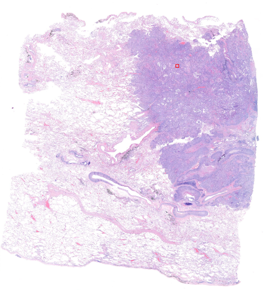
The tiny little red square that you see there corresponds to this zoomed in image:

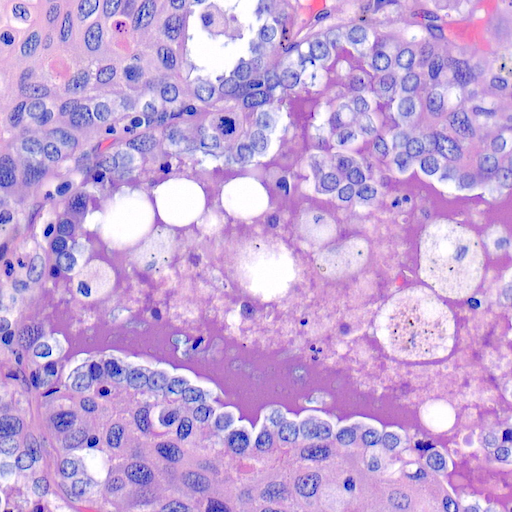
As you can see those images are massive, and analysing them requires time and effort. Not only that, each tissue is different, the above was for lung, but the skin looks more like this:

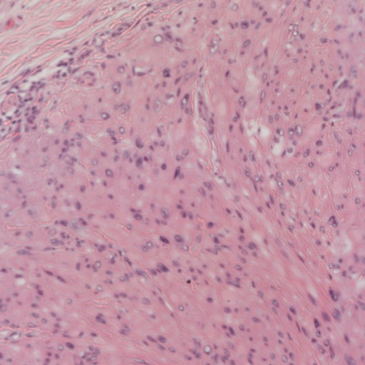
And worse than that, there are several different ways to stain the cells. This is the cheapest staining which is called Hematoxylin and Eoxin, but there are others like the immunohistochemistry that creates a better distinction between tumoural and non-tumoural cells but are more expensive. The problem we tackled in the article was to detect if a given WSI corresponded to malignant tissue or not.

This type of problem can also be described in the context of Multiple Instance Learning (MIL). In a MIL setting you have to classify a bag of elements into a given class where each individual element has its own class that influences the overall class of the bag. For instance, imagine you want to give a score of how good a basketball team is. If you have Stephen Curry or Lebron James in the team the overall score goes up. The difference in the MIL setting is that you don’t know how good each player is, you just know how the team performed in the last matches. And you try to infer based on that. If you know the team scored 30 three-point shots then you may assume there is one hyperscorer and if in another match the team does not score one single three-point shot then you may be inclined to think that hyperscorer is not playing. This is the type of latent information that we try to discover in a MIL setting. By analysing bag of images we try to find some patterns in the individual images that help analyse other bags of images, without ever knowing anything specific about those images, just knowing about the whole bag.

To be more specific, what we want is to split the WSI into smaller images and be able to classify the WSI only by classifying all the zoomed in patches and then aggregating the result. If we detect one patch to be malignant, then the WSI is quite probable malignant, no matter whether the other images are malignant or not. By looking at many malignant WSI it is possible to extract patterns about the smaller patches and learn to classify those as well. One reasonable question is why? Why is useful to split the image in little pieces? Why not classify the WSI as a whole? The reason is because it is not technically possible at the moment. Training a convolutional neural network (or worse, a transformer) may require TBs of GPU RAM which is impossible right now. And even if that were possible, the amount of data to train such models will also need to be huge, which is not at the moment. The dataset we published in the article has less than 300 patients. Current AI models require billions of images for working at 512x512 resolution. Imagine what is needed for 100000x100000 resolution.

But the problem does not finish there. A MIL classification problem is something already quite studied, that is not worthy of an article. The problem is far more complicated. In a MIL setting you ignore the individual labels (they are considered latent variables) and try to infer them using Ground Truth (GT) bag-level labels. Well, what if we don’t even have a Ground Truth? That’s right, labelling medical images requires doctors, but what if we could avoid that little annoyance? What if we could use non-expert annotators instead? Instead of training with expert labels, the problem we faced was to train with annotations that were made by students. Students are cheaper and are more prone to collaborate in research. If we could somehow learn when each of the students is making a mistake we could correctly obtain the GT by asking several students. That is called crowdsourcing.

To sum up, the problem we face is to classify huge medical images were we only have access to noisy labels during training.

The solution

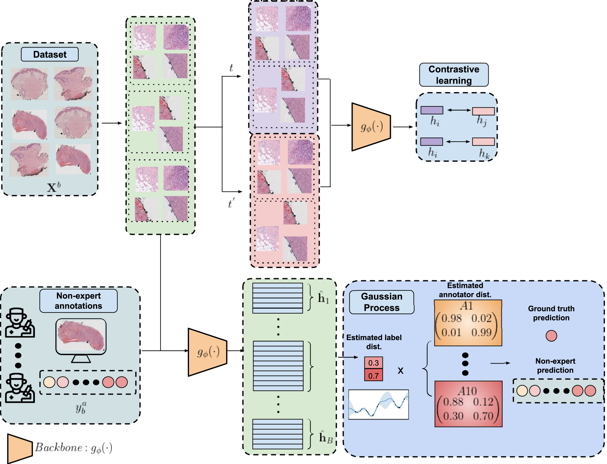
The first step to reduce the dimensionality of the problem is to train a Region of Interest (ROI) prediction algorithm. The WSIs have a lot of white pixels that can be discarded. To extract such ROIs the experts annotated some regions and then a network trained on that subset of WSI was used to predict the ROI of the rest of the dataset. After that the WSIs were splitted into 512x512 images at 10x magnification. As a reference, the maximum level of magnification is 40x, so we also reduced the dimensionality here by working with more pixelated patches. That is this part of the diagram:

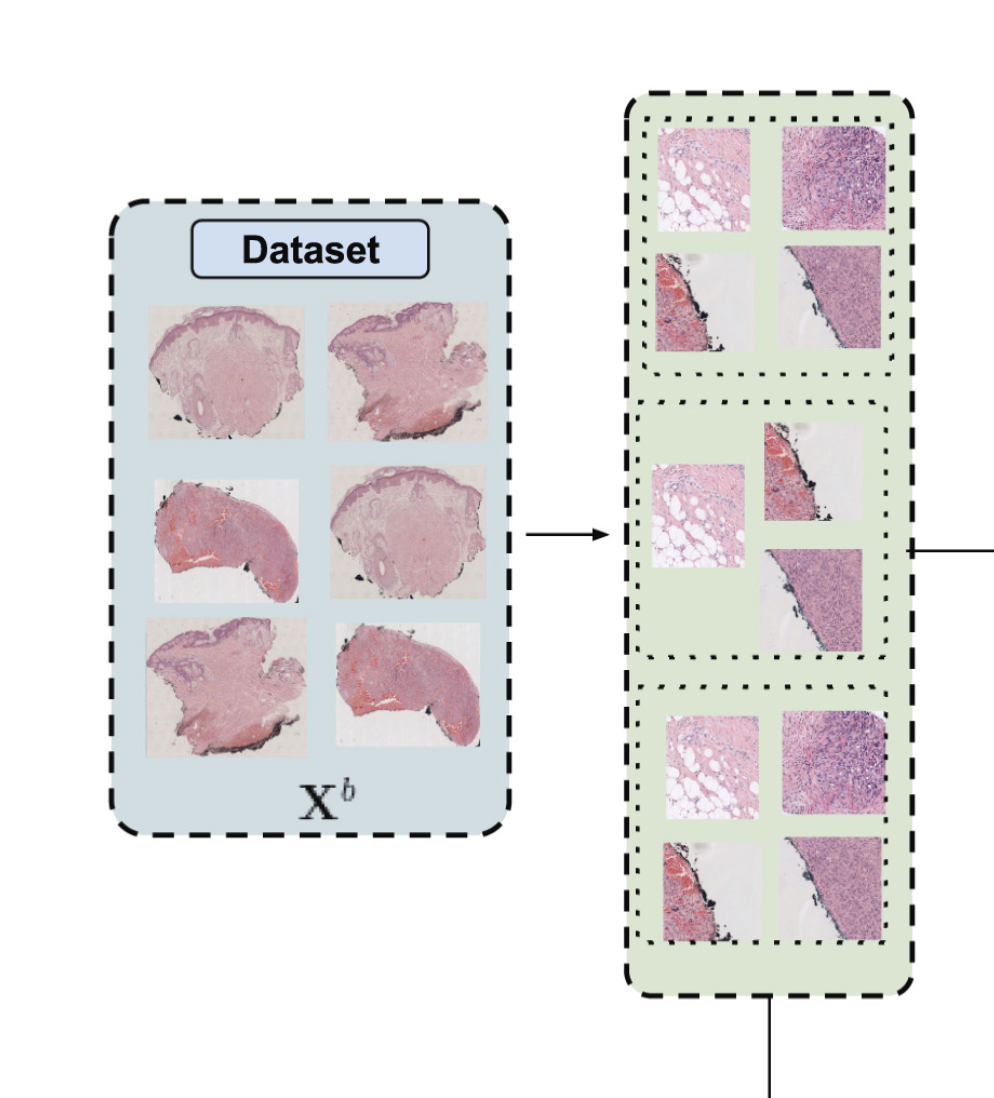
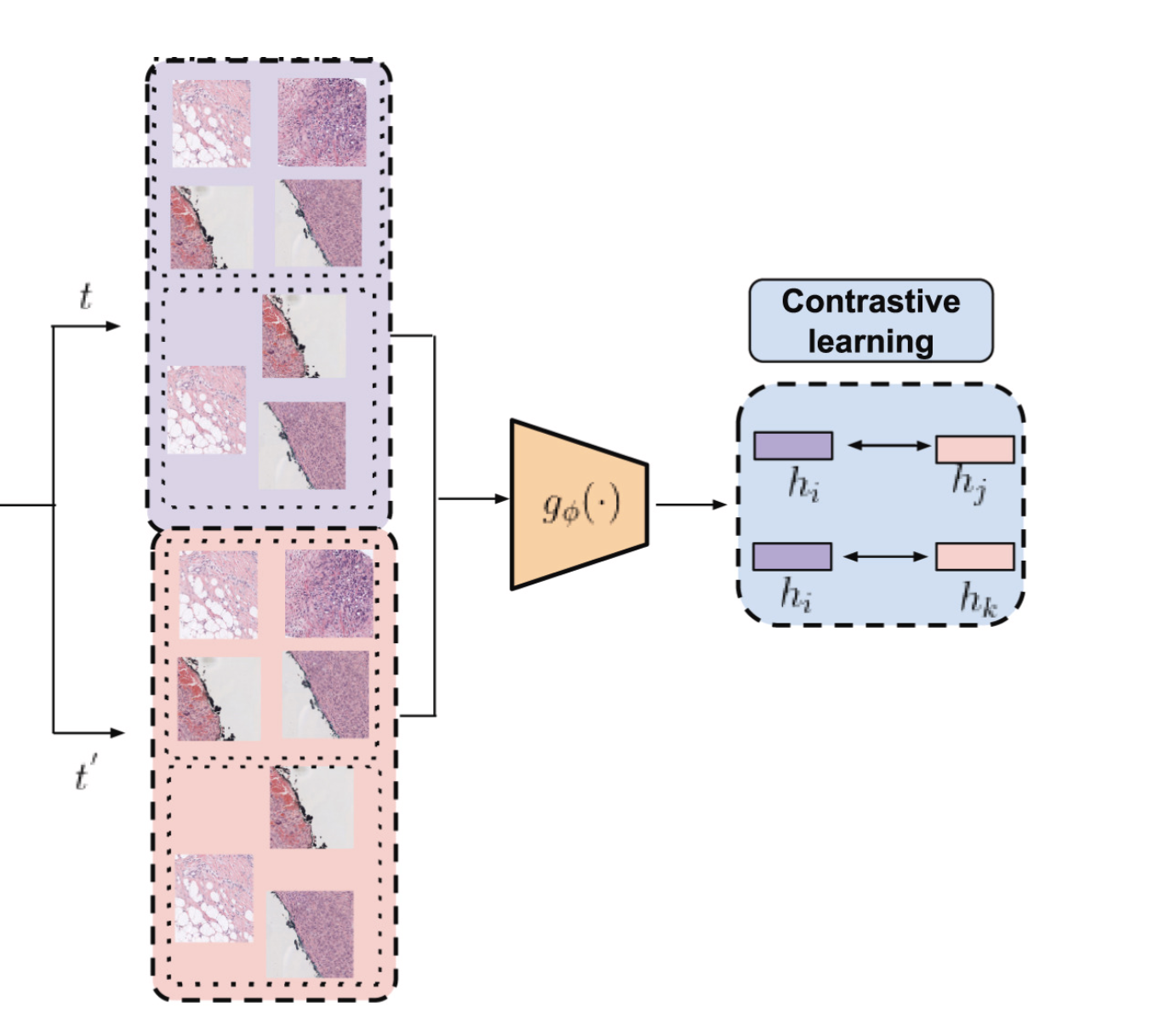
The next step to reduce even more the dimensionality was to train a convolutional neural network in an unsupervised manner to obtain feature vectors. This way we could reduce 512x512 images into vectors of dimension 256. Even more than that, we aggregated the feature vectors of each image inside a WSI. So we went from between 100 and 1000 images to just one single vector of 256 numbers. That unsupervised method is called SimCLR. It consists of a very special loss called normalized temperature-scaled cross-entropy loss (NT-Xent). Mathematically it can be expressed like this:

The $\bf{h}$ are the feature vectors. Unlike other common losses, this loss is not computed independently for each item in the batch and then aggregated. This loss takes into account every element in the batch and is computed for each positive pair and then aggregated. A positive pair is a pair of images that should be considered similar, and a negative pair one that should be considered different. For instance, an image and its reflection or rotation are considered similar while two images of two different patients are considered dissimilar. This way by minimizing this loss one is maximizing the similarity of positive pairs (numerator) at the same time that it is minimizing the similarity between negative pairs (denominator). Where the similarity is measured using cosine similarity. The result is that the network is training to have a separable latent space. Such property is very useful for training classifiers on that latent space. The rest of the parameters in that formula are not quite relevant. The $\tau$ is the temperature but is always fixed at $0.5$ and the $S$ is the batch size which is limited by the RAM you have, so there is not much room for improvement there. Surprisingly, we found that a batch size of 256 gives better results than one of 512. This is surprising because in the original SimCLR article they stated that anything below 512 was useless. Well, it is not.

We have covered the top right of the diagram:

With that we overcome the limitations of the MIL setting and reduce the problem to a strongly-supervised one. The next step is to solve the crowdsourcing problem, which is the last part of the diagram:

To solve it we can model the problem as a bayesian network. In a bayesian network you have observable variables and latent variables. All the variables influence each other in some way, either as a prior distribution or a dependency relation or in many other ways. The key here is the Bayes Theorem. It lets us go forward and backward. If by knowing the distribution of A we can know the distribution of B, then the reverse also holds. If we know B we can get A. This means that if the output depends on some latent variable we can infer some information about that unknown variable by observing the output. In our case, the bayesian network is visualized in this diagram:

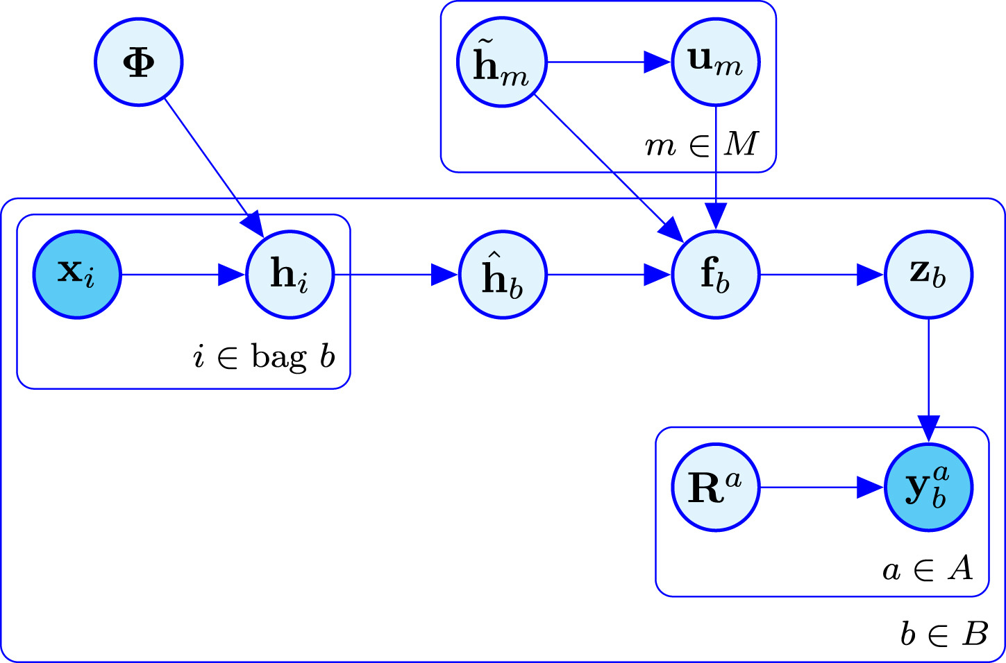
Here $\bf{x}_i$ are the input images and $\bf{y}_b^a$ are the non-expert annotations. Those are the only two variables that are observable. And everything that is in between must be inferred in order to obtain a model that predicts labels from images. There are two parts to distinguish in this diagram. The crowdsourcing part and the Gaussian Process part. One models how each annotator behaves while the other adds extra latent variables to make the model more robust and scalable. The easiest to understand is the crowdsourcing part. There are true labels $\bf{z}_b$ for each bag $b$ and each annotator $a$ has a confusion matrix $\bf{R}^a$ that describes the probability that they make a mistake. We don’t know such probabilities neither the true labels, but we aim for discovering them based on the data. Such thing is possible whenever the majority of the annotators are better than random and not adversarial annotators. But even if there is only one adversarial annotator, that is, someone that says exactly the opposite of the truth, it is possible to identify it and correct their labels.

The Gaussian Process part is adding an extra latent variable called $\bf{f}_b$ that is more or like a hidden layer in a neural network. It is supposed to capture the relations between new samples and all the training samples so that it can provide a prediction based on similarities computed with some kernel function. Since computing the covariance matrix with respect to all the training data has cubic cost, there is yet another latent variable called inducing points or $\bf{u}_m$ that is supposed to summarise all the content of the training data into just a reduced set of points. There is a lot of theory behind this way of modelling, if any of you is interested in all the maths you can refer to the original LIGO paper that designed this model. Or if you want to know about gaussian processes you can refer to the original article of the scalable version of the GPs.

To summarise in a simple phrase the whole method, we are reducing dimensionality by first extracting a ROI, then applying a pretrained network to obtain latent variables, and after that we are applying a crowdsourcing method to classify those extracted features learning from noisy labels. Believe or not, this is not an original method, it is just “a mechanical combination of existing methods”. Or that is what a reviewer said.

Curiosities

The problem and the solution are explained with more detail in the paper. I would like this blog post to contain information that is not published, to reveal other more enjoyable facts that are not told anywhere. During this project we found many results that were not only counterintuitive but sometimes outright against the theory. Since there is the possibility that those facts were due to some implementation detail and not due to the method itself, we didn’t publish them, or didn’t highlight them too much.

The first interesting fact is that the initialization of the parameters of the GP affected the result in a very dramatic way. Going from 1 to 2 make the model improve quite drastically. That is surprising because the model must converge to the same value no matter how you initialise it. And it is even more surprising that such a little change can affect so dramatically the output. Contrary to neural networks, GPs have much less parameters. And changing the initialization of just two of them can change the result. This is something that does not happen on other problems or is very difficult to replicate, but it happened to us.

The second interesting fact, and this one was the matter of many discussions, is that the crowdsourcing model is sometimes better that a model trained with the expert labels. That is, using non-expert labels can bring better results than using expert labels. At first this caused some commotion. The other authors thought that this implied the experts were not so expert after all. And we even thought about not publishing the article, because such a result could invalidate the test labels. However, the experts are indeed experts and this fact has nothing to do with that. The reason why a model trained on non-experts labels outperforms a model trained on expert labels is not because the labels are worse, but because the model is worse. In machine learning there is one thing called the bias-variance tradeoff where you can obtain better results in a regression problem by reducing the variance even if your model is systematically worse (high bias). In regression one can reduce variance by using ensembles. Without improving the quality of the members of the ensemble, the overall result improves if you perform the mean. In crowdsourcing something similar happens, but this time it is classification and not regression, and instead of bias and variance we have precision and recall. What we found is that the model trained on experts has a higher recall. And that has a lot of sense. Doctors have a tendency to diagnose an illness even if not present because the alternative is worse. It is better to do more tests than to say one is healthy wrongly. For that reason, training with expert labels tends to have that tendency too. The magical part of using crowdsourcing is that it increases precision out of thin air. By averaging the annotations of several people a similar effect as with an ensemble is achieved. This way, even though all the individual non-expert annotators have lower precision than the experts, when combining them they achieve higher precision. So, the conclusion is that doctors are very cautious and to obtain a more precise answer one should ask several doctors.

The third fact is a consideration about the research process itself. When we started this project we were quite sure that the method was going to give better than random results easily. Wrong! This database was absurdly difficult to work with. We had to perform a very exhaustive hyperparameter search and even when doing so it was not enough the first time. Initially we were not going to use SimCLR. We tried to use the crowdsourcing method alone. But the method was designed for low dimensions and so we had to try a way to simplify things. And even after finding SimCLR it was not enough because it provided feature vectors for images, not for WSIs. In the end, we made some very arbitrary decisions like simply averaging the vectors instead of using some attention mechanism. And after all that was done, we still had to perform an exhaustive search over the hyperparameters of the model. When we began the project we thought we could iterate at least three times, and we barely manage to iterate once. That is why the model only tackles the binary case even though the database is multiclass. And that is why our model is not end to end. Those two ideas were supposed to be done after achieving a simple baseline. But achieving such simple baseline ended up consuming all the time.

The last amazing fact is that the validation set does not correlate with the test set. Truly inspiring isn’t it? The metrics we obtained in the validation set were around 60% or so while the metrics from train and test were around 70 and 80%. And the best performing model in the validation was rarely the best performing model on the test set. That is why the metrics we report on the article are so low sometimes. Not because the model itself is bad in the test, but because the best set of hyperparameters in the validation set is not the best set in the test. Since you cannot use the test set for hyperparameter tuning, the result ended up being worse than expected. If I were to start the project again, I would choose the split to have similar images on all of the splits while not mixing the patients. The current split makes it impossible to infer useful information. It is even better to do the tuning on the training than on the validation set. This is a reason not to deploy any model trained on this database, since you cannot be sure it won’t drift on new patients.

The reviewing process

We are used to hear many scientis complain about the peer review system and I now know why. All the reviewers wanted was for us to cite their articles. They criticised that we didn’t mention this or that article. And after looking at all the proposals we found that they all had the same author in common, what a coincidence! This is a recurring theme, in the other article I have the same happened. It is not something strange. Even the editor in chief advises you not to give up to the citation abuse in their mails.

Yet not every request is about citing them, some are about “pinta y colorea”. Little changes about how the figures are made or the colours we use. For instance, if you look at the bayesian network above you will see it is blue. That was a request from the reviewers. Initially it was black and white like in the thumbnail of the post but that change was proposed “To enhance the originality and clarity of the method’s approach”.

Worse than that is when the reviewers simply ask you to improve your english. The article has been supervised by more than five people who have been working on this for decades and have several hundreds of articles published and the reviewer still thinks the english is improvable. I sometimes think the reviewers didn’t even read the article and criticised based on the title and little more.

Conclusion

Research has its ups and downs, but I like it. The happiness that fills your heart when your method is finally improving and giving good results is very different than any other emotion. It is different than selling a product to a client or developing a new feature in an app. It feels as if you are discovering a new world. Although when the time passes you look back and think “What a useless piece of … did I do there?”. That is progress though, improving means what you did is now obsolete. Many people is afraid of change. I am not one of them. I embrace it. Whenever I have the possibility of learning something new I try. Even if that means learning that all your efforts in the past year are now a commodity. That is compensated by the amazing new thing you just discovered. I hope I will always be discovering new and better technology and science for that is what improves the quality of life of everybody.